Posts tonen met het label Kimball. Alle posts tonen

vrijdag 27 januari 2017

Slowing Changing Dimensions (SCD) explained

Introduction

Changes in data in a data warehouse (Slowing Changing Dimension principle) is a key concept of a data warehouse. If you track the changes in a data warehouse it is possible to go back in time and see what happened with the data. That is an advantage. The disadvantage is that complexity is added in the ETL process and in the reports.

In this blogpost I'll explain the fundamentals of Slowly Changing Dimensions with a small example in PowerPivot and Excel.

Data model

Below, the data model is shown with two dimensions and a fact. The dimensions are a product dimension, in which products are categorized and one date dimension (granularity month). The fact table is a simple fact table that has a number of keys to the dimensions DimCalendar and DimProduct. There is a measure NetRevenue present.


Example data

For this article, I have created a small example in Excel where a product with a ID 4 draws some attention, the hairdresser. This product is in the category of transportation. This is accidentally or it may have some other reason. But, most logical is that the product is in the wrong category.


If we handle this in a graph with the categories Personal Care and Transportation together, it looks like this.


We look to the category Personal Care only and it looks as follows.


Slicing the data with the category "Transportation" will show this graph.


Slowly Changing Dimension 1 (TYPE I)

Meanwhile, we found out (in this scenario) that the categories are not good. We see that the product Hairdryer falls into the wrong category. We change the category to Transportation for  Hairdryer. This looks like this:


If we change the categories (hairdryer is personal care) then this has effect on the charts. It changes the charts and not just at the moment of the change but also retroactively. Even if we correct data now, everything is changed in the past. This may be desirable (most likely in this particular example), but it may also have undesirable effects in other situations.

For example, it can also take place at the moment that a company changes their range of products. What happens then? New products and categories are created, products may have moved to another category, products are made inactive or deleted in the source systems. In short, it depends on what concern is the source of the kind of change. Is there an error or is a strategic choice the reason to change the products and categories. It is difficult to guess the true reason of a change in the data.

Let's see what if a product changes from category. Product4, the hairdryer has changed category Transportation to Personal Care. The following occurs. It seems that the change generated additional revenue in the year for the category Personal Care. Good news for the sales manager who is responsible for the category Personal Care.


However, there is also a change that takes place in the chart for the category Transportation. Unfortunately, the sales manager will have to do with a lesser bonus this year. He or she may enjoy less bonus. The turnover has moved from the category Transportation to Personal Care.


Slowly Changing Dimension 2 (TYPE II)

May be it is desirable what I have descibed in the former paragraph (a logical correction of the categories), but it can also have undesirable effects, for instance when another series of products is introduced. Then you want the figures as they were and these should be calculated differently in contrast with the new product series. How can we achieve this? Suppose we make the product dimension SCD2? What happens then? If there is a change in the source system then both the old record is preserved and a new record is created. See below on the right side There is a new record created for hairdryer and a new record ProductID 8. Suppose that a new record is loaded into the data warehouse? See this event on the left. At 201801 there will be a sales record with a revenue of 500.


And here you can see now that nothing has changed in 2017 for both categories? Below the composite chart with NetRevenue both personal care as well as transportation. In 2017 there is absolutely nothing that changed, but we had this in SCD1 too. The total of the categories remained the same.


Let's look at the NetRevenue of the underlying products in each category. We also see no change for 2017. 


And Personal Care chart looks as follows for 2017


Slowly Changing Dimension 3 (TYPE 3)

There is another variant that can be very useful, namely SCD3. This is a variant which can be used in the case of a comparison between an old and a new situation. Let us consider a change in the producthierarchy. Let's take the example above with products and categories. In the above case, the producthierarchy can change at a given time (rightly or wrongly). Suppose we now want to see the new data with the old producthierarchy. In other words, it would be like there is no new producthierarchy. What would have looked the numbers? And they also want to know how the figures in the past with the new product hierarchy would have seen if there had always been a new producthierarchy. The old product hierarchy has never existed. Two varieties :
  • With an old producthierachy you want to see both old and new data.
  • A new product hierarchy can see both the old and the new data.

In the data model, you can fix this. I've added an extra column and the old one is renamed to Category Before and the after producthierarchy we call CategoryAfter.


Now we can therefore make a distinction between 'for the change' and 'after the change'. In the example below, there is now a new slicer, namely CategoryAfter. With this we can now switch between the new and the old situation and compare them to see what has changed.


Conclusion

In this article, we discussed the impact of a change in dimension data . In addition, various options put forward to be here to deal with in order to achieve a desired result. The suggestions made are not applicable to every situation, "it depends." It is necessary to check each situation.

Greetz,

Hennie

zondag 15 maart 2015

Big Data : Data Obese (Part I)

Introduction

We are buried under the amount of information that we collect. Especially the amount of data we refer to as big data information. This information is mostly unstructured or semi structured like JSON or XML. We need on an information diet. How do we handle this?

In addition, some companies (Cloudera)  has already announced that the end of the data warehouse will happen when Hadoop is full grown. I'm still not convinced, especially in the short and medium term. Hadoop is an eco system that is under development and it has lots of potential.


Why a (structured) data warehouse?

Why do we have a (structured) data warehouse? You'd almost forgotten in the Big Data violence that we hear and read daily. Let's go back to the basics. A data warehouse is the place where we can store all information of an organization (and beyond) in a structured way. Structure is important in this statement. This fact has many advantages. The data has been optimized for complex queries. It has been cleaned (ETL) and a labelled (metadata) such as: It is a varchar and it is always 50 characters wide.

Relieving a sourcesystem can be an important advantage too. For example, if there is no data warehouse then, each data mart or a brief report must have access to the source system. The one-time retrieval of the data in an isolated environment can thus relieve the production systems.


But the main advantage is the fact that a data warehouse can integrate data from different sources. Based on business keys used by the organization so you can integrate for example, sales, purchasing and production (vertical columns) again make horizontal. You collect and integrate all departments.

And, if you want you want do it completely right,  then you have to make sure that you save the history data from the source systems properly. Often people will think you mean the old data, but it is not. The point is that you save the changes of the data in the source systems. This has advantages, namely that you have the central place and your data warehouse is the truth for all corporate data. After all, you have saved the state of a source system at any point in time. So now  you can time travel, "How my report looked at the time April 1, 2013?". The report will show the position of the data at that specific time. Subsequent changes have no effect. No more guesswork by stating that changes in the data provide other figures in the reports (if you do not save changes). It also has other advantages namely that you are 'auditable', you can re-generate new insights on old data and you can analyze processes by example you have registered status changes (process mining).


How does Big data fit into this?

But now the big question : "how does big data fit in this story?". The question is what we mean by big data and that is difficult. It has become such a huge container concept that it is not entirely clear what exactly is big data. Looking at the 3 Vs will see it is a lot of data, which are very diverse and that also goes fast. Suppose we assume a (enterprise) data warehouse,  there are complex business rules and integration issues it is not expected that real-time processing is possible. This is simply not easy to achieve. Assuming this situation : speed (real time) is less important, we still hold about two aspects that may be important in a big data data warehouse: The amount of data and the variety.

For the amount of data, we could realize a Hadoop solution that stores the unstructured data. Because there is no schema, you can store data quickly in a Hadoop cluster. And, you can store all information without you know the schema of the data. Imagine that your datastructure  has changed, You have to drop and recreate the table in a RDBMS and that is not needed with Hadoop. 

There is no schema data (we do not have data types such as varchar or integer). In short, when reading the data from the Hadoop cluster, then we have to define a schema. Defining the schema can be defined very broadly. The script (mapper) determines what is the schema. For example, you can run the script Text ETL where you are looking for patterns. But for example with Hive, that is part of the ecosystem Hadoop make a schema on the data files in HDFS. This is also called "Schema-On-Read '.


But let's just focus on unstructured information such as email, reports, Word documents or files that have a bit more structure such as error logs or web logs. So basically data without metadata. How can we analyze this? We can use text ETL. You can search for patterns, for example, taxonomies or ontologies. Below is an example of a taxonomy:

Transport
  • Auto
    • Manufacture
      • Honda
      • Fiat
      • Porsche
    • Type
      • SUV
      • Sedan
      • Station
  • Aircraft
    • Manufactur
      • Airbus
      • ....

Suppose you want to analyze this sentence:

"We drove and we passed a Porsche and a Volkswagen on the highway"

If we handle this with a taxonomy then the following may come from:

"We drove and pased the Porsche / Manufacturer past a Volkswagen / Manufacturer on the highway / road"

Then we could save this information as a Name - Value pair:

Manufacturer: Porsche
Manufacturer: Volkswagen
Road: Highway

And in this way, it looks a bit more structured. And this would be the time to load it in the data warehouse and combine with other structured data. This is not the only way but there are many more. Eg Name-Value processing, or Homografic resolution, or example List processing. These are all techniques you can use to filter out patterns in the data (to schematizing).

An architecture that can handle this could be this :


The data lands from structured sources in stagingarea that is structured and the unstructured data lands in a data lake (Hadoop). Then the structured information is loaded into an Enterprise Data Warehouse (EDW), processed and reported by BI tooling. The unstructured data is stored in a data lake and analyzed in an analytical platform with all kinds of tooling such as R or with the power series of Microsoft. This is a more explorative process (discovery). The results are written back into the data lake, after which this data can be read again into the EDW. The EDW also provides display data to the analytical platform in order to enrich the unstructured data. So there are multiple loops in this architecture. And that is generally so with big data architectures. It is heterogeneous environment with various tooling that do what they are good at.


Conclusions

So this is a way to reduce the amount of data that make data less 'data obese'. It is important that we find ways to extract information from the enormous information piles that we can use in analytical platforms and can add value to structured (enterprise) data warehouses.

Greetz,

Hennie 

zondag 21 september 2014

SSAS : Multicurrency Problem (Part I)

Introduction

Suppose, you're working for an international company in Europe and this company has many branches across the world. These branches are located in countries with different currencies. Therefore, this multinational company book her transactions in local currencies. This blogpost is about how to handle multicurrency in a SQL Server Analysis Services environment.

Now, the first thought solution is to introduce two columns in the fact table, in case you've a Kimball data warehouse, off course.  But, suppose there are region managers in countries who are responsible for the sales in other countries. And the region manager reports in it's own currency (let's say American Dollars). The region manager is also responsible for Mexico. The currency of Mexico is Pesos. Now, the region manager wants to see the sales in American Dollars of the countries he is responsible for. The pesos should be converted into American Dollars. The head office of this multinational company is in the Netherlands and they report in Euros.

This blog post is about collecting the sold products and services in a local currency and convert it to any other currency that is desired. So, this is in my opinion the most flexible solution. In this way, we can handle very easily organization changes, for instance, like that region management is moved from USA to Mexico. Now, the American Dollars and Pesos can now easily consolidated into Pesos.

Overall, there are a couple of scenarios possible:
  1. Data is collected in one currency and it must be converted into multiple currencies (website scenario).
  2. Data is collected in multiple currencies and it must be converted into one currency (headquarter scenario).
  3. Data is collected in multiple currencies and it must be converted into multiple currencies (subsidiary and multiregion scenario).
In this blogpost I'll discuss option number 3.

And, there are a couple of solutions:
  1. Create multiple currency columns (EURO, USD, etc) in the fact and convert the local currency into the columns. The advantage is that it's simple. Disadvantage is that it's fixed.
  2. Convert the different currencies into an base currency during the ETL, and build multicurrency conversion in the cube. This is more complex than number 1 option.
  3. Import the different currencies into the cube and convert the currencies at query time. This is the most complex conversion solution but also a neat one!
I'll take number 3!

For this blogpost I've used the book "Expert Cube Development with SQL Server 2008 Analysis Services" by Chris Webb, Alberto Ferrari and Marco Russo. In Chapter 7 an explanation is given about MultiCurrency problems. Now as you are googling about MultiCurrency the proposed MDX Script isn't the best generated solution (in any way for the Many2Many way) and better and more performant solutions are available. I'll blog about them in future blogpost. So be aware!

For this blogpost I've used SQL Server 2008 R2 and Excel 2013.

MultiCurrency Problem

In this blogpost I'll write down a solution that worked for me in a lab experiment. In future blogposts I'll investigate improvements of the base solution I'll present here. In the base solution, there a couple of tables needed:
  • FactOrderLine.
  • DimProduct.
  • DimDate.
  • CurrencyRate.
  • Currency.
I've created a database "MultiCurrency" and ran the script below.

USE [MultiCurrency]
GO

DROP TABLE [dbo].[FactOrderLine]
GO

DROP TABLE [dbo].[CurrencyRate]
GO

DROP TABLE [dbo].[DimProduct]
GO

DROP TABLE [dbo].[DimDate]
GO

DROP TABLE [dbo].[DimCurrency]
GO

CREATE TABLE [dbo].[DimCurrency](
 [Currency_ID] [varchar](50) NOT NULL,
 [Currency_Name] [varchar](50) NULL,
 CONSTRAINT [PK_Dimcurrency] PRIMARY KEY CLUSTERED 
(
 [Currency_ID] ASC
)WITH (PAD_INDEX = OFF, STATISTICS_NORECOMPUTE = OFF, IGNORE_DUP_KEY = OFF, ALLOW_ROW_LOCKS = ON, ALLOW_PAGE_LOCKS = ON) ON [PRIMARY]
) ON [PRIMARY]
GO

CREATE TABLE [dbo].[DimDate](
 [Date_ID] [int] NOT NULL,
 [Day] [varchar](50) NULL,
 [Month] [varchar](50) NULL,
 CONSTRAINT [PK_DimDate] PRIMARY KEY CLUSTERED 
(
 [Date_ID] ASC
)WITH (PAD_INDEX = OFF, STATISTICS_NORECOMPUTE = OFF, IGNORE_DUP_KEY = OFF, ALLOW_ROW_LOCKS = ON, ALLOW_PAGE_LOCKS = ON) ON [PRIMARY]
) ON [PRIMARY]
GO

CREATE TABLE [dbo].[DimProduct](
 [Product_ID] [int] NOT NULL,
 [Product_Name] [varchar](50) NULL,
 CONSTRAINT [PK_DimProduct] PRIMARY KEY CLUSTERED 
(
 [Product_ID] ASC
)WITH (PAD_INDEX = OFF, STATISTICS_NORECOMPUTE = OFF, IGNORE_DUP_KEY = OFF, ALLOW_ROW_LOCKS = ON, ALLOW_PAGE_LOCKS = ON) ON [PRIMARY]
) ON [PRIMARY]
GO

CREATE TABLE [dbo].[CurrencyRate](
 [CurrencyRate_ID] [int] IDENTITY(1,1) NOT NULL,
 [Date_ID] [int] NULL,
 [Currency_ID] varchar(50) NULL,
 [Rate] [float] NULL,
 CONSTRAINT [PK_CurrencyRate] PRIMARY KEY CLUSTERED 
(
 [CurrencyRate_ID] ASC
)WITH (PAD_INDEX = OFF, STATISTICS_NORECOMPUTE = OFF, IGNORE_DUP_KEY = OFF, ALLOW_ROW_LOCKS = ON, ALLOW_PAGE_LOCKS = ON) ON [PRIMARY]
) ON [PRIMARY]
GO

CREATE TABLE [dbo].[FactOrderLine](
 [OrderLine_ID] [int] IDENTITY(1,1) NOT NULL,
 [Date_ID] [int] NULL,
 [Product_ID] [int] NULL,
 [Currency_ID] varchar(50)  NULL,
 [Amount] [money] NULL,
 CONSTRAINT [PK_FactOrderLine] PRIMARY KEY CLUSTERED 
(
 [OrderLine_ID] ASC
)WITH (PAD_INDEX = OFF, STATISTICS_NORECOMPUTE = OFF, IGNORE_DUP_KEY = OFF, ALLOW_ROW_LOCKS = ON, ALLOW_PAGE_LOCKS = ON) ON [PRIMARY]
) ON [PRIMARY]
GO


INSERT INTO [dbo].[DimCurrency]
           ([Currency_ID],
      [Currency_Name])
     VALUES
           ('EUR', 'EUR'),
     ('GBP', 'GBP'),
     ('USD', 'USD'),
     ('MEX', 'MEX')

-- [DimDate]
INSERT INTO [dbo].[DimDate]
           ([Date_ID],
      [Day],
      [Month])
VALUES
           (20140921, 'Sunday', 'September'),
     (20140922, 'Monday', 'September'),
     (20140923, 'Tuesday', 'September'),
     (20140924, 'Wednesday', 'September'),
     (20140925, 'Thursday', 'September'),
     (20140926, 'Friday', 'September'),
     (20140927, 'Saturday', 'September')

--[DimProduct]
INSERT INTO [dbo].[DimProduct]
           ([Product_ID],
      [Product_Name])
     VALUES
           (1, 'Bicycle'),
     (2, 'Car'),
     (3, 'Motor'),
     (4, 'Bus')

INSERT INTO [dbo].[CurrencyRate]
           ([Date_ID]
           ,[Currency_ID]
           ,[Rate])
     VALUES
           (20140921, 'EUR', 1.0), --EUR
     (20140922, 'EUR', 1.0), --EUR
     (20140923, 'EUR', 1.0), --EUR
     (20140924, 'EUR', 1.0), --EUR
     (20140925, 'EUR', 1.0), --EUR
     (20140926, 'EUR', 1.0), --EUR
     (20140927, 'EUR', 1.0), --EUR
     (20140921, 'GBP', 1.25), --GBP
     (20140922, 'GBP', 1.27), --GBP
     (20140923, 'GBP', 1.30), --GBP
     (20140924, 'GBP', 1.32), --GBP
     (20140925, 'GBP', 1.40), --GBP
     (20140926, 'GBP', 1.21), --GBP
     (20140927, 'GBP', 1.22), --GBP
     (20140921, 'USD', 0.77), --USD
     (20140922, 'USD', 0.80), --USD
     (20140923, 'USD', 0.62), --USD
     (20140924, 'USD', 0.90), --USD
     (20140925, 'USD', 0.66), --USD
     (20140926, 'USD', 0.33), --USD
     (20140927, 'USD', 0.90), --USD
     (20140921, 'MEX', 0.06), --MEX
     (20140922, 'MEX', 0.10), --MEX
     (20140923, 'MEX', 0.05), --MEX
     (20140924, 'MEX', 0.11), --MEX
     (20140925, 'MEX', 0.12), --MEX
     (20140926, 'MEX', 0.14), --MEX
     (20140927, 'MEX', 0.15) --MEX
GO

INSERT INTO [dbo].[FactOrderLine]
           ([Date_ID]
           ,[Product_ID]
           ,[Currency_ID]
           ,[Amount])
     VALUES
           (20140922, 1, 'EUR', 5), 
     (20140922, 1, 'EUR', 7.7),
     (20140922, 2, 'GBP', 8.95),
     (20140925, 1, 'EUR', 5),
     (20140923, 2, 'USD', 100),  -- 0,62 * 100 = 62
     (20140921, 1, 'EUR', 500),
     (20140925, 1, 'EUR', 1000),
     (20140926, 4, 'MEX', 300)
GO

SELECT D.Currency_Name, Sum(F.[Amount])
FROM FactOrderLine F
LEFT OUTER JOIN [DimCurrency] D ON F.Currency_ID = D.Currency_ID
GROUP BY D.Currency_Name


Now start SQL Server Analysis Services and create a Datasource:

1. Create a New project in SQL Server Analysis Services.

2. Name it MultiCurrency and press OK.

3. Create a Datasource by richtclicking in the in the Solution Explorer (on the right side of Microsoft Visual Studio).

4.  The DataSource Wizard is started and press Next.

5. Create a new connection by pressing New.

6. Enter . at the server name and select the right database "MultiCurrency".

7. Press Next.

8. Select Use the Service Account at the Impersonation Information Window.

9. Enter "dsMultiCurrency" at the Data Source Name.


The next step is creating a Data source view:


10. Right click in the Solution explorer on Data Source Views. (on the right side of Microsoft Visual Studio)

11. Press Next when the wizard opens.

12. Select the Datasource and press Next

13.  Press Next in the Name Matching window.

14. Select all tables in the Available objects, press > button and press Next.

15. Name the DataSourceView "dsvMultiCurrency".


This is the Data Source View :


Okay let's create the dimensions:

16. In Solution Explorer (on the right side of Microsoft Visual Studio), right-click Dimensions, and then click New Dimension. The Dimension Wizard appears.

17. On the Welcome to the Dimension Wizard page, click Next.

18. On the Select Creation Method page, verify that the Use an existing table option is selected, and then click Next.

19. On the Specify Source Information page, verify that the dsvMultiCurrency data source view is selected.

20. In the Main table list, select DimDate.

21. Click Next.

22. On the Select Dimension Attributes page, select the check boxes next to the following attributes:
  • Day
  • Month

23. Change the setting of the Day attribute's Attribute Type column from Regular to Day of week.To do this, click Regular in the Attribute Type column. Then click the arrow to expand the options. Next, click Date > Calendar > Day of Week. Click OK.


24. Do this also for Month. Change Attribute Type to Month.

25. On the Completing the Wizard page, in the Preview pane, you can see the Date dimension and its attributes.

26. Click Finish to complete the wizard.

27. In the Solution Explorer, in the MultiCurrency project, the Date dimension appears in the Dimensions folder.

28. On the File menu, click Save All.

Now do the other dimensions. Don't forget to make special adjustments for the Currency dimension.

For the Currency dimension:

29.   Change the setting of the CurrencyID attribute's Attribute Type column from Regular to Currency ISO Code.To do this, click Regular in the Attribute Type column. Then click the arrow to expand the options. Next, click Currency>Currency>Currency ISO Code.

30. The same approach for Currency Name.


31.. On the File menu, click Save All.

Now let's define the cube.


32. In Solution Explorer, right-click Cubes, and then click New Cube.

33. On the Welcome to the Cube Wizard page, click Next.

34. On the Select Creation Method page, verify that the Use existing tables option is selected, and then click Next.

35. On the Select Measure Group Tables page, verify that the dsvCurrency data source view is selected.

36. Click Suggest to have the cube wizard suggest tables to use to create measure groups.


37. Click Next.

38. On the Select Measures page, review the selected measures in the Currency Rate and the Fact Order Line measure group.


39. Click Next.

40. On the Select Existing Dimensions page click Next.

41. Click Next.

42. On the Completing the Wizard page, change the name of the cube to MultiCurrency.

43. Click Finish to complete the wizard.

44. On the File menu, click Save All.

Before using the Business Intelligence wizard we have to make some adjustments in the model:

45. Change the IsAggregatable property to False for the key attribute.

46. Change the Type property of the measure group "Exchange Rate"  to ExchangeRate (Best practice).

Now it's time to start the Business Intelligence Wizard :

47. Right click on the cube in the Solution Explorer and Click on " Add Business Intelligence".

48. Click Next.

49, Click on "Define Currency conversion" in the Choose Enhancement window and press Next.

If you did not process the cube earlier the following window appears


Now let's process the cube and see if there are some changes in this window:


Now this looks better...

50. Press Next.

51. Select Amount in the "Select Members" window and press Next.


52.  In the "Select Conversion Type" window it's possible to select the currency conversion. Make sure that Many-to-Many is selected. Press Next.


53. In the "Define Local Currency Reference" Window a link between the local currency and the transaction is selected.


54. In the "Specify Reporting Currencies" Window select All of the Reporting Currencies and press Next.


55. On the Completing the Wizard page, in the Changes pane, you can see the changes that are being made by the Business Intelligence wizard to the Datasource view, dimensions and the Cube. Press Finish.


The dimension Usage Tab looks like:


A table in the Datasource View is added:


And on the Calculations Tab a MDX Script is added (snippet):


56. In the File Menu,  Click Save All.

57. Deploy and process the Cube.

Now we are done making changes to the cube. Now it's time to check whether the adjustments are doing the right calculations.

58. Start Excel and create a new excel sheet. For this blogpost I used Excel 2013.

59. Go to the Data Tab and select "From Other sources", Select "From Analysis Services"

60. Enter . in the Servername in the Connect to Database Server window.

61. Make Sure that the database "MultiCurrency" and the Cube "MultiCurrency" is selected and press Next.

62. Press Next.

63. Press OK.

If everything went ok a pivot table is created in excel.

64. Now let's select the Amount in the PivotTable fields and put them in the Measures pane, Select currency ID of the Dimcurrency dimension and put that in the Rows Pane and Select the Currency ID of the Reporting Currency and put that in the Columns Pane.

The window now looks like this:


On the left you can see the initially entered currencies and in the columns are the converted amounts to the reporting Currencies shown. Now we have to check whether these are correct values.

For example, lets take the 100 USD. There is one order with a value of 100 dollar on September 23, 2014 and the currency conversion rate on September 23, 2014 is 0.62. So the 100 * 0.62 = 62 dollar. And that is correct.

If we drag the DateID (I know) into the Rows Pane the following values are shown:


Let's double check whether one these values are correct.

Suppose we take the orderlines of September 22, 2014 and compare these with the cube..There are three Orderlines:
  • Two bikes for 5 and 7.7 euro (hmmm bit cheap)
  • One Car for 8.95 Britisch Pounds


The Currency rates on that day are:


I checked the calculations manually in Excel and the calculations are correct.


Conclusion

In this blogpost I've shown the conversion of currencies at query time in the Cube. Now, although this is great, there are some drawbacks about this solution. The CurrencyRate and the DimCurrency are not built according to the Kimball starschema theory. For instance, the key of the dimCurrency dimension is not integer but varchar. So, although it looks great, I'll investigate whether if things could be improved.

According to the blog of Chris Web this solution is not a very performant solution, unfortunately. The solution above takes about 9 seconds on the AdventureWorks Database.

Other references:

Greetz,
Hennie


zondag 4 maart 2012

Four different datamodeling methods

Introduction
Most of the time, 3NF are datamodels that are used in transactional systems like an orderentry application. For datawarehousing we had until a couple of years ago the (historized) 3NF and the starschema. Since a couple of years there are some new kids in the datawarehouse town: Datavault modeling and Anchor modeling. These datamodels try to deal with the disadvantages of 3NF and starschemas.

We are starting to learn that the starschema is more an end user datamodel that is easily understood by end users. It's a high performance model. Datavault modeling and Anchor modeling are more focussed on storing the right information in such a way that you achieve agility, speed of development and auditability. There are more reasons but i don't want to elaborate too much.

At first i wanted to write down a successor of my first blogpost about Anchormodeling but soon the blogpost became more and more an overview of the four types of data modeling techniques. I hope to write more about anchormodeling in next blogposts.

In this exercise i'll use the 3NF datamodel of the AdventureWorks2008LT Database . This is a simplified database of the large SQL Server AdventureWorks 2008 database. You can find this LT database on the site Microsoft codeplex. There isn't a SQL Server 2012 version available yet, as far as i  know. I'll transform this 3NF datamodel into a Datavault model (As i've blogged earlier), a anchor model and a starschema model.

Adventureworks2008LT  (3NF)
Below a representation of the 3NF datamodel as i've analyzed from the Adventureworks2008LT database. There are a couple of transaction tables (SalesOrderHeader and SalesOrderdetail) present and some master data tables (Customer, Productdescription, productcategory, etc). At first sight there seems no reference data in the diagram.


Adventureworks2008LT (3NF) in more detail
Below the database in more detail. I've decided to leave the errorlog and buildversion out of the models.


The Datavault model
As mentioned in my earlier blogpost i've used Quipu as a tool to generate the datavault model from the Adventureworks2008LT database. This tool can be downloaded, for free. The datavault model that is generated by Quipu is a typically source datavault model. You can find more information about this discussion at the blog of Ronald Damhof.

Now, the model that is generated is shown in the diagram below. The blue tables are the links, the orange tables are hubs and the yellow ones are the satellites. I've organized the diagram in a way that it looks like as much as possible as the Adventureworks2008LT 3NF model.


At first sight, you'll see that the number of tables are more than the 3NF model. That  is because the relations have become a table (link), the busineskeys have become a seperate table (hub) and the descriptive fields are stored in another table (sat). In my opinion the main advantage of this model is that you can increase agility and speed of development by separating the relations, business keys and the descriptive fields. Auditability seems to me a derived advantage of the agility argument: a historized 3NF datawarehouse datamodel is also auditable. But because the datavault model is more flexible that the 3NF model you can achieve the auditabilty much easier and faster than the historized 3NF datamodel.

The Anchor model
Below you can see a first draft of the Anchor datamodel. In my former post i've briefly explained a piece of the anchor modeling technique. I'm currently investigating this modeling technique for usage in my projects. It seems an interesting technique. The agility is pushed to the extreme because every field in a source table is a table in the anchor model. You can imagine that this enhances maximum flexibility.


The Adventureworks2008LT 3NF model is exploded into a huge number of tables in the anchor model. A good naming convention is very very appropriate. Even better, a tool should be available to manage the tables. In a future post i'll show the tables that are created and i can tell you now that the 9 tables in the 3NF model are about 100 tables in the anchor model (depending of the number of attributes in a table in the source model).

The diagram is created on the site http://www.anchormodeling.com/ and although it's a great solution and it looks great there are some disadvantages. It took me quite some time to create the datamodel.

The starschema
Below an example is shown of a starschema based on the Adventureworks2008LT 3NF datamodel. There are a couple of directions possible depending on the business process you're supporting. I've chosen to model it like this but you could also combine the SalesOrderHeader and the SalesOrderDetail in one fact. Or you could remove the snowflake table Category and move it to the fact. So depending on your (future?) business question you determine the starschema model.

In this example i've decided to split the SalesOrderHeader and SalesOrderDetail table in two facts. The SalesOrderHeaderDD is the link between the two facts. There are a couple of  difficult relations in the AdventureWorks2008LT 3NF model:
  • The relation product-Category.
  • The n:m relation between the productmodel and the Productdescription entity.
  • The relation between customer and address (CustomerAddress).


I've decided not to model the Customeraddress in the model. I've also decided to model the other difficult relations in the same way as the 3NF datamodel, resulting in a snowflake relation and a bridge table solution. Off course there are other decisions possible.

Conclusion
First, this blogpost started in my mind with a successor of the anchormodeling blogpost but later on i've decided to rewrite the blogpost to a overview blogpost of the four datamodels i'm interested in. I hope it gives an overview of the models.

So in my opinion we have now the following options to model a datawarehouse:

  • Historized 3NF model.
  • Datavault model.
  • Anchormodel.
  • Starschema.

From these options it seems that for a data storage foundation the best solution is datavault model or the anchor model. For enduser reporting and cube design the starmodel seems the most optimal solution. The main problem of the historized 3NF model is that the cascading changes that can happen and therefore this model is not the best option (in my opinion).

Greetz,

Hennie

donderdag 23 juni 2011

SSAS/Kimball : building a multivalue dimension construction in SSAS (part II)

In my former post i'll already explained the background for this post. If you didn't read this than i would advice reading this first post before reading this article. In this article i'll explain about building a multivalue dimension in SSAS (MM dimension). This post covers the following subjects:

  • Prerequisites.
  • Building a cube.

    Prerequisites
    Below you can see a script i've been using for building a cube. At the end of the script i've added a couple of facts/events.  So when we will quering this cube the following results should be shown for departments:
    • Department A : 3
    • Department B : 2
    • Department C : 2

    And for the locations:
    • Location 1 : 1
    • Location 2 : 2
    • Location 3 : 2

    First create a database and execute the following script:

    IF  EXISTS (SELECT * FROM sys.objects WHERE object_id = OBJECT_ID(N'[dbo].[TestFact]') AND type in (N'U'))
    DROP TABLE [dbo].[TestFact]
    GO

    CREATE TABLE [dbo].[TestFact](
        [TestFactID] [int] IDENTITY(1,1) NOT NULL,
        [FK_Date_Key] [int] NOT NULL,
        [FK_Location_Key] [int] NOT NULL,
        [TestFactCount] [int] NOT NULL
    ) ON [PRIMARY]
    GO

    ----
    IF  EXISTS (SELECT * FROM sys.objects WHERE object_id = OBJECT_ID(N'[dbo].[Location]') AND type in (N'U'))
    DROP TABLE [dbo].[Location]
    GO

    CREATE TABLE [dbo].[Location](
        [Location_Dim_key] [int] NOT NULL,
        [Location_Code] [int] NOT NULL,
        [Location_Description] [varchar](50) NOT NULL
    ) ON [PRIMARY]
    GO

    ----
    IF  EXISTS (SELECT * FROM sys.objects WHERE object_id = OBJECT_ID(N'[dbo].[Department]') AND type in (N'U'))
    DROP TABLE [dbo].[Department]
    GO

    CREATE TABLE [dbo].[Department](
        [Department_Dim_key] [int] NOT NULL,
        [Department_Code] [int] NOT NULL,
        [Department_Description] [varchar](50) NOT NULL
    ) ON [PRIMARY]
    GO

    ---
    IF  EXISTS (SELECT * FROM sys.objects WHERE object_id = OBJECT_ID(N'[dbo].[Bridge_Location_Department]') AND type in (N'U'))
    DROP TABLE [dbo].[Bridge_Location_Department]
    GO

    CREATE TABLE [dbo].[Bridge_Location_Department](

        [Bridge_Location_Department_ID] [int] IDENTITY(1,1) NOT NULL,
        [FK_Location_Key] [int] NOT NULL,
        [FK_Department_Key] [int] NOT NULL,
        [Valid_From] [date] NOT NULL,
        [Valid_Until] [date] NOT NULL
    ) ON [PRIMARY]
    GO

    ---
    IF EXISTS (SELECT * FROM sys.objects WHERE object_id = OBJECT_ID(N'[dbo].[DimDate]') AND type in (N'U'))
    DROP TABLE [dbo].[DimDate]
    GO

    CREATE TABLE [dbo].[DimDate](
    [Date_dim_key] [int] NULL,
    [Date_Year] [int] NULL
    ) ON [PRIMARY]
    GO

    ---

    INSERT INTO dbo.Department (Department_Dim_key, Department_Code, Department_Description)
    VALUES (1, 1, ' Department A' ),(2, 2, ' Department B' ), (3, 3, ' Department C')

    INSERT INTO dbo.Location (Location_Dim_key, Location_Code, Location_Description)
    VALUES (1, 1, ' Location 1' ),(2, 2, ' Location 2' ), (3, 3, ' Location 3')

    INSERT INTO dbo.Bridge_Location_Department (FK_Location_Key, FK_Department_Key, Valid_From, Valid_Until)
    VALUES (1, 1, '2011-01-01', '9999-12-31' ),
    (2, 1, '2005-01-01', '9999-12-31' ),
    (2, 2, '2005-01-01', '9999-12-31' ),
    (3, 3, '2005-01-01', '9999-12-31' )

    INSERT INTO dbo.DimDate
    VALUES (1,2000),
    (2, 2001),
    (3, 2002),
    (4, 2003),
    (5, 2004),
    (6, 2005),
    (7, 2006),
    (8, 2007),
    (9, 2008),
    (10, 2009),
    (11, 2010),
    (12, 2011),
    (13, 2012),
    (14, 2013),
    (15, 2014),
    (16, 2015)


    INSERT INTO [MultiValueDimension].[dbo].[TestFact]
               ([FK_Date_Key]
               ,[FK_Location_Key]
               ,[TestFactCount])
    VALUES
               (7, 1, 1),
               (7, 2, 1),
               (8, 3, 1),
               (9, 3, 1),
               (9, 2, 1)


    Building a cube
    Okay, now we have to build a cube based on the tables created in SQL Server. Kimball calls this a multivalue dimension (actually it's a variant on the multivaluedimension, in my opinion). Microsoft calls this a many-to-many dimension (MM). Marc Russo published a great whitepaper on this subject. Many-to-many dimension (MM) is a better name for this subject. What can we say about Many-to Many dimension construction in relation to the case we are building:
    • There are two measure groups needed.
    • There are two dimnsions needed.
    • The bridge Location Department table will be Intermediate Measure Group. The intermediate Measure Group is the measure group that relates the MM dimension to the regular dimension In this case it relates the location to the department dimension.
    • Location is the intermediate dimension.


    Designing this in the cube designer shows this picture:


    So how does this looks in the dimension usage tab of the cube designer?


    As said earlier in the post: location and department are the dimensions. Testfact and the bridge location department table are the measure groups. So when we check the results in the browser we see the following results for the locations:


    And for the departments:


    The total is still 5 but adding the departments subtotals manually is equal to 7!!!

    And this is as predicted at the beginning of this post. So we have reached nirvana. Well not quite yet. What about history?  What if a location do not exist anymore between departments and locations? What if locations shift from locations to other departments? You want to count your facts at right departments in a correct timeline! I'll blog about this in the future.

    So, this is it for now.

    Greetz,
    Hennie

    dinsdag 14 juni 2011

    SSAS/KIMBALL: modeling a N:M relation between dimensions (part I)

    Hi,

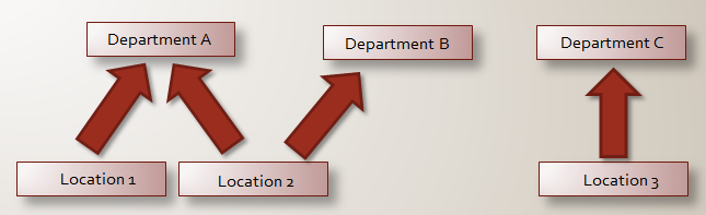
    During the development of a dashboard for a customer i've a awkward problem. The situation is like this: There are events in the every daily business (fact) and these events can happen on certain locations (physical) locations. These locations can be shared by different (logical) departments.  So conceptually you have something like this:


    And if you model this in a Bachman diagram (3NF) it will look like this:


    So there are two standard entities and one associative entity has been added for handling the n:m relation. This way n:m relations can be easily modeled in 3NF. So the values for the department table will be :
    1. Department A
    2. Department B
    3. Department C
    The values for the location table are:

    1. Location 1
    2. Location 2
    3. Location 3
    And the associative table "Department_Location" contains :

    1. 1 (Department A), 1 (Location 1)
    2. 1 (Department A), 2 (Location 2)
    3. 2 (Department B), 2 (Location 2)
    4. 3 (Department C), 3 (Location 3)
    And you could introduce a valid_from and a valid_to (as in temporal modeling) where you can check the validity whenever the record is valid or not. Relations exists and can no longer exist at some point in time.

    A first assumption of me was modeling the location and the department seperately (the grain of the fact is at location level):


    So the grain is at Location level and therefore a 'simple' dimension is enough. But the fact can happen at different departments (e.g. in case of location 1) and therefore i introduced a bridge table. So the key of the fact table is pushed to the bridge department table and the department dimension key is also pushed to the bidge department table. But wait a minute.....there is a drawback of this modeling solution. You can't see whether which location belongs to which department, unless a fact has happen. If a fact didn't happen you can't determine whether a location belongs to a department. So i needed a better solution than this.

    The solution
    So studying kimball's book : "the datawarehouse lifecycle toolkit, second edition" shows me a example on page 270, paragraph "many-values dimensions with bridge tables". In this example a account dimension and Customer dimension is used with a bridge table. A weighting factor can help adding facts to the right customer. But i'm my situation i don't know how the facts are related to the department. Sometimes 99% of the facts belongs to the departments and sometimes less facts and this is not sure.  So in my case a proper modeling solution is this :


    In this case it's possible to determine which location belongs to which department.

    Kimball recommends adding a valid_from and a valid_to column to the bridge table (as i already explained in the 3NF example) because a relation can exist at a certain point in time and they can no longer exist at some moment.

    Next time i'll explain how to build this in SSAS.

    Greetz,
    Hennie